I've updated my Offensive Decision% formula to include Offensive Rebounds. A field goal attempt is now only considered one 'decision' if the player does not rebound the attempt. So the denominator now subtracts Offensive Rebounds x Shot% in an estimation of how many offensive rebounds a player makes on their own missed field goals. Here's the entire formula:
Here are the current results for the NBA, with those playing 500 minutes or more.
Praise for The Basketball Distribution:
"...confusing." - CBS
"...quite the pun master." - ESPN
NCAA team offensive efficiency impacts
I have previously done work on estimating how much statistics (specifically, the Four Factors + 2 more) impact efficiency. My prior method was lazy and inaccurate at adjusting for Strength of Schedule. The new method adjusts each factor rating differently. For the math, scroll to the bottom* EDIT: Yes, the total numbers do not EXACTLY equal (Adjusted Offensive Rating - League Average Offensive Rating), but they are close (R^2 of .99, to be concise).
But here's what you really want.
NCAA adjusted offensive four factors
*The original method took (Deductive Efficiency - Deduced efficiency with league average stat) and multiplied this by (Adjusted Efficiency / Raw Efficiency). The new method is a little more complex. I found out that each stat didn't impact efficiency as much as I thought, since each factor interacts with one another. I found the following:
While predicting change in efficiency (minus average), the following weights occur: eFG&FG+=1.065833, TO%+=1.088916, OR%+=0.935664, FTR&FT+=0.38507
Each individual output would have to be multiplied by these coefficients. However, I still needed to adjust for strength of schedule. To do this, I subtracted Adjusted - Raw Offense for each team to get their Schedule Adjustment Factor. I then weighed each of the four factors so that they would sum to one (fg=0.306672, to=0.313314, or=0.269218,ft= 0.110796). Here's an example of how eFG%&FG% look:
eFG&FG+=1.065833 * [(Deduced Efficiency - Deduced efficiency with average eFG% and FG%) + .306672*Schedule Adjustment ]
NCAA player offensive ratings
Just put together another round of player offensive ratings - data via KenPom.com. It adjusts for quality of defense and usage% - the final number is an estimate of how efficient an average team's offense would be with the player on the court.
Here's the results
Here's the results
2010 Tourney "All-or-nothing" Ratings
This is using my pre-tournament LRMC simulation from last year. See my last blog post for the method,. I still haven't come up with a good name for it.
How does "effective likelihood of doing better than statistically expected" sound?
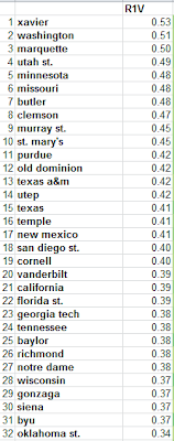
The first-round component gives us the most meaningful information (as the later rounds heavily favor better teams). Let's take a look at the results:
1) Xavier: as a 6-seed, beat 11-seed Minnesota and 3-seed Pittsburgh
2) Washington: as an 11-seed, beat 6-seed Marquette and 3-seed New Mexico
3) Marquette: lost to the (more-volatile) Washington
4) Utah St: lost to Texas A&M (who was just 0.07 lower in volatility)
5) Minnesota: lost to (highest-volatility) Xavier
other notables: the official Cinderella of 2010, Butler, was #7 (volatility of 0.48). Also, Cornell (who beat the 5 & 4 east seeds as a 12-seed), was ranked 19, with 0.4.
On to the second round:
1) West Virginia: made it to the Final-Four as a two-seed.
2) BYU: fell to Kansas St, who was 5th in volatility
3) Duke: Won the tournament...
4) Kentucky: Didn't make it past West Virginia, but succeeded as a (statistically) overrated team
5) Kansas St: Fell to Butler in the Elite 8 - pulled through in a pretty tough bracket though (statistically)
other notables: Butler is the highest-ranked 5-seed in 2nd-round volatility.
The third round doesn't tell us much new information, although Duke is the highest-ranked team here (in a bracket that statistically favored Kansas).
Anyways, the information here is hard to quantify, but I think some important things can be learned, especially from the first-round component!
How does "effective likelihood of doing better than statistically expected" sound?
here's the first, second and third (r1, r2, and r3)
The first-round component gives us the most meaningful information (as the later rounds heavily favor better teams). Let's take a look at the results:
1) Xavier: as a 6-seed, beat 11-seed Minnesota and 3-seed Pittsburgh
2) Washington: as an 11-seed, beat 6-seed Marquette and 3-seed New Mexico
3) Marquette: lost to the (more-volatile) Washington
4) Utah St: lost to Texas A&M (who was just 0.07 lower in volatility)
5) Minnesota: lost to (highest-volatility) Xavier
other notables: the official Cinderella of 2010, Butler, was #7 (volatility of 0.48). Also, Cornell (who beat the 5 & 4 east seeds as a 12-seed), was ranked 19, with 0.4.
On to the second round:
1) West Virginia: made it to the Final-Four as a two-seed.
2) BYU: fell to Kansas St, who was 5th in volatility
3) Duke: Won the tournament...
4) Kentucky: Didn't make it past West Virginia, but succeeded as a (statistically) overrated team
5) Kansas St: Fell to Butler in the Elite 8 - pulled through in a pretty tough bracket though (statistically)
other notables: Butler is the highest-ranked 5-seed in 2nd-round volatility.
The third round doesn't tell us much new information, although Duke is the highest-ranked team here (in a bracket that statistically favored Kansas).
Anyways, the information here is hard to quantify, but I think some important things can be learned, especially from the first-round component!
Team Volatility
This is going to be a shortish post considering the amount of new analysis I'm introducing, but I would like to start offering some tools to help predict even the strangest of occurrences. For example, it would have been statistical folly to predict Northern Iowa or Cornell to win as many games as they did in 2010; I want to predict the next Cornell!
So let's go in order of depth.
First, basic probabilities: teamrankings.com has some phenomenal pre-selection simulation projections for the tournament, giving individual probabilities for each team making it to round X.
From these we can find AVERAGE PROJECTED WINS: simply sum together each of the 6 probabilities to find the mean-expected wins each team will have in the tournament.
From this, we can do some theory: given that team x wins at least y games, how many wins will they THEN be projected to have; I call this "Average Projected Wins with X games secure." This would be estimated like so:
=Y games won + sum(probabilities of the rest of the tournament)/(probability of winning Y games)
So for two games secure, the math would be:
=2 + sum(probabilities of winning the 3rd,4th,5th, and 6th games)/probability of winning in the second round)
From this, we can get a hybrid statistic, that I like to call Volatility: this is the marginal wins gained from winning any specific round of the tournament, TIMES the probability of winning that round. We do this by subtracting "X games secure" from our starting average (zero games secure).
For example, one team's volatility in the first round would be:
=[(2-win secure average wins) -( 0-wins secure average wins)] * odds of winning those first two games
The first three rounds are the ones that tell us the most information, l
ater rounds are skewed by higher-quality teams having much higher odds of winning the games beforehand. On the right are the top ten teams by "first round volatility," considering the projected fielding of teams.
This tells us, roughly, which team will benefit the most if they can overcome early obstacles. A better utilization of this method would be to subtract from the ESPN National Bracket "average wins" rather than my statistical "zero wins secure average." This gives us a better picture of which team will do better than expected by most, and therefore, which team will help you destroy everyone in your office pool!
Offensive Decision%
Finally, some good old fashioned statistics that don't have really good theory behind them!
Often-times, when I'm watching a basketball game, I mentally determine who is making the most good decisions and the most bad decisions on offense.
So here's a basic metric of what my eyes see, and I call it Offensive Decision %. It basically measures, poorly, Good Offensive Decisions / Total Offensive Decisions.
=(FGM + Assists + .44 * FTM) / (FGA + Assists + TO + .44 * FTA)
And here's the top NBA players (as of earlier this week) with median minutes played or more.
Estimated defensive rating formula, with Usage% !
EDIT/UPDATE: This formula, like Dean Oliver's is based on some good theory, but as I have examined it more, it is a very poor measure of defensive success. If you need a quick fix, the following explains player defense better than the formula described:
(Points Allowed On Court / Possessions Played) - (Points Allowed Off Court / Possession Off-Court)
Woo! This one took a lot of work, but I think I have all of the theoretical errors taken care of. It's very similar to Dean Oliver's box-scoreformula, but with a few important adjustments:
(Points Allowed On Court / Possessions Played) - (Points Allowed Off Court / Possession Off-Court)
Losing Larry Drew II
EDIT: I accidentally named Strickland in the paragraph on defensive plus-minus rather than Drew. Now fixed.
The North Carolina Tar Heels just lost Larry Drew II, transferring after playing some pretty decent basketball (according to that article).
Let's take a moment and look at Larry Drew's estimated offensive impact.
Using 15% of the Tar Heels' possessions for 57.5% of each game, with their lowest Offensive Rating, I estimate that losing Drew will bring Carolina's 'Raw' Offensive Efficiency up to 107.88 (from 106.45). Depending on how you look at it, Drew's absence would add between 1.4 and 1.5 points per 100 possessions to Carolina's 'Adjusted Offensive Rating'.*
Also, I ran StatSheet's plus-minus data and found that (weighted by minutes played) while Drew was on the court, Carolina averaged a point margin of 2.3 per 40 minutes. With his replacement point guards on the court, they averaged 10.8 points per 40 minutes. To this effect, Drew's on-court presence hurt Carolina by 8.5 points per 40 minutes.
But Larry Drew's main claim to fame was his defensive prowess. There are no truly good defensive stats for players like Drew, but we have to assume that he contributed some to Carolina's defense. Let's try to take a closer look:
Some quick stats from his Pomeroy page: I'll rank him among the three players who run point the most (Marshall, Strickland, and Drew).
Defensive Rebound%: Drew takes the lead at 9.3%, in close second is Strickland's 8.7%. Marshall isn't far behind at 7.4%
Block%: Ha! Marshall is the only one recording noticeable blocks, with 0.3%.
Steal%: Drew posts an impressive 2.7, but Strickland and Marshall have him beat at 3.1 and
Fouls Committed per 40: While fouling helps in some situations, Carolina's best Four-Factor stat is how few times their opponent gets to the line. This will likely only improve, as Drew's
modest 3.4 is bested by Marshall's 2.3 and Strickland's 2.6.
Defensive Plus Minus: Not going to rank players (takes too long to get these numbers), but with Drew on the court, Carolina allowed 40.9 points per 40 minutes. Off the court, Carolina allowed only 28.0 points per 40 minutes. That means that with Drew on the floor, Carolina did 12.9 points per 40 worse on defense.
It's never a very good idea to only use plus minus when looking at players, but NET +/- can tell us some reasonably accurate things about the effect of substituting players. As long as Carolina can emotionally push through this, losing Drew could actually win them an extra game or two. I just pray that the boys stay out of foul trouble and don't get fatigued now that a lot of minutes have to be filled.
Furthermore, I think that I would personally stick with Strickland, not Marshall. While Marshall posts an insane assist rate of 42.8 (compared to Strickland's 12.6), I'll take Strickland's TO% of 18.4 over Marshall's sloppy 32.9 any day.
That is all!
That is all!
*One way of adjusting is just adding the 1.4 to the raw numbers. But if I use the ratio of UNC's Adjusted Efficiency to Actual Efficiency (1.034), the impact goes from -1.43 to -1.47.
NCAA Love...or How I Learned To Keep Worrying About Maryland Not Making It...
The following my listing of projected NCAA seed (from RPIforecast.com) versus LRMC seed (LRMC ranking + .75):
NCAAlove.PDF
Maryland still gets the short end of the stick, and Oklahoma St. gets too much love.
NCAAlove.PDF
Maryland still gets the short end of the stick, and Oklahoma St. gets too much love.
Subscribe to:
Posts (Atom)
Followers
About Me
- Nathan
- I wish my heart were as often large as my hands.