There are several teams who simultaneously impress statistical rankings, but do not impress poll-rankings.
Here are all the teams who are in the top-25 of at least one of my three favorite systems --and not ranked in either major poll--: by Ken Pomeroy's efficiency margin, Raymond's Ratings (basically SRS, if you're familiar), and GA Tech's Bayesian Logistic Regression Markov Chain.
Top-25, The-Humans-Are-Unimpressed
(bold indicates a computer system being similarly unimpressed, italics indicate top-10 computer rating)
-Washington (P10, 19-9) - #13 Pomeroy, #8 Raymond, #6 LRMC
Washington has had a particularly tough time away from home, losing two of three on neutral courts (by single digits to Kentucky and Michigan State), and losing six of eleven on the road (only once by double-digits). At home, on the other hand, the Huskies won their first thirteen before putting up a non-characteristic eFG% of 39.7 against Washington St. on Sunday, losing by eleven. Their blowout wins prove a marked inconsistency, as they absolutely beat up on decent teams. Washington beat top-100 Pomeroy teams Oregon, Long Beach St, Arizona, UCLA, USC, Cal (twice), and Stanford, by an average of 18.4 points. I won't give up on them (as Pomeroy similarly encourages you to do) because of this, and their demolishing of Arizona and their quality road performance at UCLA.
-Maryland (ACC, 18-11) - #16 Pomeroy, #16 Raymond, #32 LRMC
Four of these losses include: An 8-point road loss at Duke, an 11-point road loss at Carolina, a 9-point neutral loss to Pittsburgh, and 8-point road loss to Villanova. Their overall strength of schedule is low since 1/3 of their season has been against sub-200 teams. This is evident in the extremely flawed RPI, who knocks Maryland down to #83. Ouch. If these guys win the ACC tourney, I would expect them to win a couple in the big dance...but the odds are not in their favor to get that first step.
-West Virginia (BE, 18-10) - #18 Pomeroy, #18 Raymond, #19 LRMC
Exactly half of WVU's ten losses have come against top-25 Pomeroy teams, and they have wins against Vanderbilt, Cincinnati, Purdue, and Notre Dame. Their Pomeroy strength of schedule, as one might expect, is 2nd in the country.
-Belmont (ASun, 27-4) - #20 Pomeroy, #24 Raymond, #8 LRMC
Belmont is an interesting case. We have a very low sample size of decent competition with these guys - they've only played three games against tougher opponents than #106-Pomeroy East Tennessee St. In fact, only eleven of their thirty-one games have been against top-200 Pomeroy teams. At any rate, their only losses have come against decent opponents (save Lipscomb), on the road, by an average of only seven points.
-Illinois (B10, 18-11) - #21 Pomeroy, #22 Raymond, #20 LRMC
The Illini have been extremely inconsistent this season. While they have lost to Illinois-Chicago on a neutral court, they beat tough opponents in Maryland, Wisconsin, Gonzaga, and North Carolina. Also, they've had to deal with the nation's 6th-highest string of opponents (by Pomeroy's metric).
-Cincinnati (BE, 22-7) - #24 Pomeroy, #28 Raymond, #34 LRMC
Cinci is at least somewhat recognized by humans, as they received the 32nd most votes in the AP poll this week. Their seven losses have come from teams with an average ranking of 19-Pomeroy.
-Marquette (BE, 18-11) - #25 Pomeroy, #26 Raymond, #27 LRMC
Marquette has had an unfortunate schedule. They've lost to neutral-court Duke by 5, road-Pittsburgh by 8, road-Lousville by 1, road-Nova by 5, road-Notre Dame by 5, and road Georgetown by 9. While the humans might not be impressed, just from those numbers alone, a statistical-minded Nathan Walker would call Marquette a top-25 team.
-St. Mary's (WCC, 23-7) - #45 Pomeroy, #32 Raymond, #23 LRMC
St. Mary's inconsistency is marked by a high-high and a very-low-low. They only lost to BYU by 1 on a Neutral court, but lost to #302 Pomeroy San Diego. In between has come a few losses to good teams and beating up every other average team they encountered.
Unfortunately, some of these squads are going to be Nationally Invited, if you know what I mean. For those that make the big dance, there's a good chance they'll beat their better-seeded opponent.


Offensive Decision% version 2
I've updated my Offensive Decision% formula to include Offensive Rebounds. A field goal attempt is now only considered one 'decision' if the player does not rebound the attempt. So the denominator now subtracts Offensive Rebounds x Shot% in an estimation of how many offensive rebounds a player makes on their own missed field goals. Here's the entire formula:

Here are the current results for the NBA, with those playing 500 minutes or more.
Here are the current results for the NBA, with those playing 500 minutes or more.
NCAA team offensive efficiency impacts
I have previously done work on estimating how much statistics (specifically, the Four Factors + 2 more) impact efficiency. My prior method was lazy and inaccurate at adjusting for Strength of Schedule. The new method adjusts each factor rating differently. For the math, scroll to the bottom* EDIT: Yes, the total numbers do not EXACTLY equal (Adjusted Offensive Rating - League Average Offensive Rating), but they are close (R^2 of .99, to be concise).
But here's what you really want.
NCAA adjusted offensive four factors
*The original method took (Deductive Efficiency - Deduced efficiency with league average stat) and multiplied this by (Adjusted Efficiency / Raw Efficiency). The new method is a little more complex. I found out that each stat didn't impact efficiency as much as I thought, since each factor interacts with one another. I found the following:
While predicting change in efficiency (minus average), the following weights occur: eFG&FG+=1.065833, TO%+=1.088916, OR%+=0.935664, FTR&FT+=0.38507
Each individual output would have to be multiplied by these coefficients. However, I still needed to adjust for strength of schedule. To do this, I subtracted Adjusted - Raw Offense for each team to get their Schedule Adjustment Factor. I then weighed each of the four factors so that they would sum to one (fg=0.306672, to=0.313314, or=0.269218,ft= 0.110796). Here's an example of how eFG%&FG% look:
eFG&FG+=1.065833 * [(Deduced Efficiency - Deduced efficiency with average eFG% and FG%) + .306672*Schedule Adjustment ]
But here's what you really want.
NCAA adjusted offensive four factors
*The original method took (Deductive Efficiency - Deduced efficiency with league average stat) and multiplied this by (Adjusted Efficiency / Raw Efficiency). The new method is a little more complex. I found out that each stat didn't impact efficiency as much as I thought, since each factor interacts with one another. I found the following:
While predicting change in efficiency (minus average), the following weights occur: eFG&FG+=1.065833, TO%+=1.088916, OR%+=0.935664, FTR&FT+=0.38507
Each individual output would have to be multiplied by these coefficients. However, I still needed to adjust for strength of schedule. To do this, I subtracted Adjusted - Raw Offense for each team to get their Schedule Adjustment Factor. I then weighed each of the four factors so that they would sum to one (fg=0.306672, to=0.313314, or=0.269218,ft= 0.110796). Here's an example of how eFG%&FG% look:
eFG&FG+=1.065833 * [(Deduced Efficiency - Deduced efficiency with average eFG% and FG%) + .306672*Schedule Adjustment ]
NCAA player offensive ratings
Just put together another round of player offensive ratings - data via KenPom.com. It adjusts for quality of defense and usage% - the final number is an estimate of how efficient an average team's offense would be with the player on the court.
Here's the results
Here's the results
2010 Tourney "All-or-nothing" Ratings
This is using my pre-tournament LRMC simulation from last year. See my last blog post for the method,. I still haven't come up with a good name for it.
How does "effective likelihood of doing better than statistically expected" sound?
The first-round component gives us the most meaningful information (as the later rounds heavily favor better teams). Let's take a look at the results:
1) Xavier: as a 6-seed, beat 11-seed Minnesota and 3-seed Pittsburgh
2) Washington: as an 11-seed, beat 6-seed Marquette and 3-seed New Mexico
3) Marquette: lost to the (more-volatile) Washington
4) Utah St: lost to Texas A&M (who was just 0.07 lower in volatility)
5) Minnesota: lost to (highest-volatility) Xavier
other notables: the official Cinderella of 2010, Butler, was #7 (volatility of 0.48). Also, Cornell (who beat the 5 & 4 east seeds as a 12-seed), was ranked 19, with 0.4.
On to the second round:
1) West Virginia: made it to the Final-Four as a two-seed.
2) BYU: fell to Kansas St, who was 5th in volatility
3) Duke: Won the tournament...
4) Kentucky: Didn't make it past West Virginia, but succeeded as a (statistically) overrated team
5) Kansas St: Fell to Butler in the Elite 8 - pulled through in a pretty tough bracket though (statistically)
other notables: Butler is the highest-ranked 5-seed in 2nd-round volatility.
The third round doesn't tell us much new information, although Duke is the highest-ranked team here (in a bracket that statistically favored Kansas).
Anyways, the information here is hard to quantify, but I think some important things can be learned, especially from the first-round component!
How does "effective likelihood of doing better than statistically expected" sound?
here's the first, second and third (r1, r2, and r3)
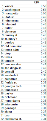


The first-round component gives us the most meaningful information (as the later rounds heavily favor better teams). Let's take a look at the results:
1) Xavier: as a 6-seed, beat 11-seed Minnesota and 3-seed Pittsburgh
2) Washington: as an 11-seed, beat 6-seed Marquette and 3-seed New Mexico
3) Marquette: lost to the (more-volatile) Washington
4) Utah St: lost to Texas A&M (who was just 0.07 lower in volatility)
5) Minnesota: lost to (highest-volatility) Xavier
other notables: the official Cinderella of 2010, Butler, was #7 (volatility of 0.48). Also, Cornell (who beat the 5 & 4 east seeds as a 12-seed), was ranked 19, with 0.4.
On to the second round:
1) West Virginia: made it to the Final-Four as a two-seed.
2) BYU: fell to Kansas St, who was 5th in volatility
3) Duke: Won the tournament...
4) Kentucky: Didn't make it past West Virginia, but succeeded as a (statistically) overrated team
5) Kansas St: Fell to Butler in the Elite 8 - pulled through in a pretty tough bracket though (statistically)
other notables: Butler is the highest-ranked 5-seed in 2nd-round volatility.
The third round doesn't tell us much new information, although Duke is the highest-ranked team here (in a bracket that statistically favored Kansas).
Anyways, the information here is hard to quantify, but I think some important things can be learned, especially from the first-round component!
Team Volatility
This is going to be a shortish post considering the amount of new analysis I'm introducing, but I would like to start offering some tools to help predict even the strangest of occurrences. For example, it would have been statistical folly to predict Northern Iowa or Cornell to win as many games as they did in 2010; I want to predict the next Cornell!
So let's go in order of depth.
First, basic probabilities: teamrankings.com has some phenomenal pre-selection simulation projections for the tournament, giving individual probabilities for each team making it to round X.
From these we can find AVERAGE PROJECTED WINS: simply sum together each of the 6 probabilities to find the mean-expected wins each team will have in the tournament.
From this, we can do some theory: given that team x wins at least y games, how many wins will they THEN be projected to have; I call this "Average Projected Wins with X games secure." This would be estimated like so:
=Y games won + sum(probabilities of the rest of the tournament)/(probability of winning Y games)
So for two games secure, the math would be:
 The first three rounds are the ones that tell us the most information, l
So let's go in order of depth.
First, basic probabilities: teamrankings.com has some phenomenal pre-selection simulation projections for the tournament, giving individual probabilities for each team making it to round X.
From these we can find AVERAGE PROJECTED WINS: simply sum together each of the 6 probabilities to find the mean-expected wins each team will have in the tournament.
From this, we can do some theory: given that team x wins at least y games, how many wins will they THEN be projected to have; I call this "Average Projected Wins with X games secure." This would be estimated like so:
=Y games won + sum(probabilities of the rest of the tournament)/(probability of winning Y games)
So for two games secure, the math would be:
=2 + sum(probabilities of winning the 3rd,4th,5th, and 6th games)/probability of winning in the second round)
From this, we can get a hybrid statistic, that I like to call Volatility: this is the marginal wins gained from winning any specific round of the tournament, TIMES the probability of winning that round. We do this by subtracting "X games secure" from our starting average (zero games secure).
For example, one team's volatility in the first round would be:
=[(2-win secure average wins) -( 0-wins secure average wins)] * odds of winning those first two games
From this, we can get a hybrid statistic, that I like to call Volatility: this is the marginal wins gained from winning any specific round of the tournament, TIMES the probability of winning that round. We do this by subtracting "X games secure" from our starting average (zero games secure).
For example, one team's volatility in the first round would be:
=[(2-win secure average wins) -( 0-wins secure average wins)] * odds of winning those first two games
The first three rounds are the ones that tell us the most information, later rounds are skewed by higher-quality teams having much higher odds of winning the games beforehand. On the right are the top ten teams by "first round volatility," considering the projected fielding of teams.
This tells us, roughly, which team will benefit the most if they can overcome early obstacles. A better utilization of this method would be to subtract from the ESPN National Bracket "average wins" rather than my statistical "zero wins secure average." This gives us a better picture of which team will do better than expected by most, and therefore, which team will help you destroy everyone in your office pool!
This tells us, roughly, which team will benefit the most if they can overcome early obstacles. A better utilization of this method would be to subtract from the ESPN National Bracket "average wins" rather than my statistical "zero wins secure average." This gives us a better picture of which team will do better than expected by most, and therefore, which team will help you destroy everyone in your office pool!
Offensive Decision%
Finally, some good old fashioned statistics that don't have really good theory behind them!
Often-times, when I'm watching a basketball game, I mentally determine who is making the most good decisions and the most bad decisions on offense.
So here's a basic metric of what my eyes see, and I call it Offensive Decision %. It basically measures, poorly, Good Offensive Decisions / Total Offensive Decisions.
=(FGM + Assists + .44 * FTM) / (FGA + Assists + TO + .44 * FTA)
And here's the top NBA players (as of earlier this week) with median minutes played or more.
Often-times, when I'm watching a basketball game, I mentally determine who is making the most good decisions and the most bad decisions on offense.
So here's a basic metric of what my eyes see, and I call it Offensive Decision %. It basically measures, poorly, Good Offensive Decisions / Total Offensive Decisions.
=(FGM + Assists + .44 * FTM) / (FGA + Assists + TO + .44 * FTA)
And here's the top NBA players (as of earlier this week) with median minutes played or more.
Estimated defensive rating formula, with Usage% !
EDIT/UPDATE: This formula, like Dean Oliver's is based on some good theory, but as I have examined it more, it is a very poor measure of defensive success. If you need a quick fix, the following explains player defense better than the formula described:
(Points Allowed On Court / Possessions Played) - (Points Allowed Off Court / Possession Off-Court)
Woo! This one took a lot of work, but I think I have all of the theoretical errors taken care of. It's very similar to Dean Oliver's box-scoreformula, but with a few important adjustments:
(Points Allowed On Court / Possessions Played) - (Points Allowed Off Court / Possession Off-Court)

Losing Larry Drew II
 EDIT: I accidentally named Strickland in the paragraph on defensive plus-minus rather than Drew. Now fixed.
The North Carolina Tar Heels just lost Larry Drew II, transferring after playing some pretty decent basketball (according to that article).
Let's take a moment and look at Larry Drew's estimated offensive impact.
Using 15% of the Tar Heels' possessions for 57.5% of each game, with their lowest Offensive Rating, I estimate that losing Drew will bring Carolina's 'Raw' Offensive Efficiency up to 107.88 (from 106.45). Depending on how you look at it, Drew's absence would add between 1.4 and 1.5 points per 100 possessions to Carolina's 'Adjusted Offensive Rating'.*
Also, I ran StatSheet's plus-minus data and found that (weighted by minutes played) while Drew was on the court, Carolina averaged a point margin of 2.3 per 40 minutes. With his replacement point guards on the court, they averaged 10.8 points per 40 minutes. To this effect, Drew's on-court presence hurt Carolina by 8.5 points per 40 minutes.
But Larry Drew's main claim to fame was his defensive prowess. There are no truly good defensive stats for players like Drew, but we have to assume that he contributed some to Carolina's defense. Let's try to take a closer look:
Some quick stats from his Pomeroy page: I'll rank him among the three players who run point the most (Marshall, Strickland, and Drew).
Defensive Rebound%: Drew takes the lead at 9.3%, in close second is Strickland's 8.7%. Marshall isn't far behind at 7.4%
Defensive Rebound%: Drew takes the lead at 9.3%, in close second is Strickland's 8.7%. Marshall isn't far behind at 7.4%
Block%: Ha! Marshall is the only one recording noticeable blocks, with 0.3%.
Steal%: Drew posts an impressive 2.7, but Strickland and Marshall have him beat at 3.1 and
Steal%: Drew posts an impressive 2.7, but Strickland and Marshall have him beat at 3.1 and
Fouls Committed per 40: While fouling helps in some situations, Carolina's best Four-Factor stat is how few times their opponent gets to the line. This will likely only improve, as Drew's
modest 3.4 is bested by Marshall's 2.3 and Strickland's 2.6.
Defensive Plus Minus: Not going to rank players (takes too long to get these numbers), but with Drew on the court, Carolina allowed 40.9 points per 40 minutes. Off the court, Carolina allowed only 28.0 points per 40 minutes. That means that with Drew on the floor, Carolina did 12.9 points per 40 worse on defense.
It's never a very good idea to only use plus minus when looking at players, but NET +/- can tell us some reasonably accurate things about the effect of substituting players. As long as Carolina can emotionally push through this, losing Drew could actually win them an extra game or two. I just pray that the boys stay out of foul trouble and don't get fatigued now that a lot of minutes have to be filled.
modest 3.4 is bested by Marshall's 2.3 and Strickland's 2.6.
Defensive Plus Minus: Not going to rank players (takes too long to get these numbers), but with Drew on the court, Carolina allowed 40.9 points per 40 minutes. Off the court, Carolina allowed only 28.0 points per 40 minutes. That means that with Drew on the floor, Carolina did 12.9 points per 40 worse on defense.
It's never a very good idea to only use plus minus when looking at players, but NET +/- can tell us some reasonably accurate things about the effect of substituting players. As long as Carolina can emotionally push through this, losing Drew could actually win them an extra game or two. I just pray that the boys stay out of foul trouble and don't get fatigued now that a lot of minutes have to be filled.
Furthermore, I think that I would personally stick with Strickland, not Marshall. While Marshall posts an insane assist rate of 42.8 (compared to Strickland's 12.6), I'll take Strickland's TO% of 18.4 over Marshall's sloppy 32.9 any day.
That is all!
That is all!
*One way of adjusting is just adding the 1.4 to the raw numbers. But if I use the ratio of UNC's Adjusted Efficiency to Actual Efficiency (1.034), the impact goes from -1.43 to -1.47.
NCAA Love...or How I Learned To Keep Worrying About Maryland Not Making It...
The following my listing of projected NCAA seed (from RPIforecast.com) versus LRMC seed (LRMC ranking + .75):
NCAAlove.PDF
Maryland still gets the short end of the stick, and Oklahoma St. gets too much love.
NCAAlove.PDF
Maryland still gets the short end of the stick, and Oklahoma St. gets too much love.
Saving My Beloved FG% from Death...
I am constantly frustrated by the current basketball community's lack of love for FG%. In Pomeroy's analysis, he looked at a very small sample of just one team. But I think it can be argued that FG% is still an important metric for two things: discussion of NBA players and of possessions.
First, a quick numerical analysis:
I took the top 310 or so NBA players and looked at how 'underrated' they are by their FG%. If we just look at the difference between eFG% and FG% we see that nearly 40% of players are underrated by 5% or more. But this is only a small part of the picture. Nobody who eyeballs the FG% of a guard thinks that a player is only shooting two-pointers. So I set up a regression for estimating eFG% via FG%. This allows us to look closer at the difference in 'roughly-expected' eFG% and eFG% itself.
Done this way, only about 10% of these players are off by 5% or more. If we get rid of the 'overrated players' (we assume that people aren't going to overrate a player's FG% in their minds), that drops to 7.7%. So at least on the player level, it's reasonable to say that FG% is pretty good for eyeballing efficiency via shooting.
Still unconvinced? Here's some more pudding:
1) FG% is useful for discussing Rebound%. To compare one team's eFG% to their OR% is not as intuitive as comparing with FG%. Field goal percent gives a better picture of 'possible rebounds' than eFG%.
2) In the same vein, FG% is more important in the discussion and analysis of what ends possessions and what doesn't.
3) I will maintain that the three-point-shot is harder to repeat. I have not done any analysis on this, but the theory is sound: the more difficult the shot, the harder it is to repeat. Therefore, to some degree, I would estimate that year-to-year FG% is a better predictor of out-of-sample eFG% than eFG% itself.
4) At least in the NBA, extremely high eFG% by a player is more likely to be from a big man; so in extreme cases of 'shooting well from the field', (which are often the important points of study), FG% is usually sufficient.
I know that none of this takes care of the two basic arguments against FG%: worse correlation with offensive efficiency, and 'just add .5*3pm from the box score!').
To that I say:
'Hey, eFG% isn't even really a percentage! It's just easier to type than Field Goal Points / (FGA * 2). I like my percentages to be out of 100, thank you!'
First, a quick numerical analysis:
I took the top 310 or so NBA players and looked at how 'underrated' they are by their FG%. If we just look at the difference between eFG% and FG% we see that nearly 40% of players are underrated by 5% or more. But this is only a small part of the picture. Nobody who eyeballs the FG% of a guard thinks that a player is only shooting two-pointers. So I set up a regression for estimating eFG% via FG%. This allows us to look closer at the difference in 'roughly-expected' eFG% and eFG% itself.
Done this way, only about 10% of these players are off by 5% or more. If we get rid of the 'overrated players' (we assume that people aren't going to overrate a player's FG% in their minds), that drops to 7.7%. So at least on the player level, it's reasonable to say that FG% is pretty good for eyeballing efficiency via shooting.
Still unconvinced? Here's some more pudding:
1) FG% is useful for discussing Rebound%. To compare one team's eFG% to their OR% is not as intuitive as comparing with FG%. Field goal percent gives a better picture of 'possible rebounds' than eFG%.
2) In the same vein, FG% is more important in the discussion and analysis of what ends possessions and what doesn't.
3) I will maintain that the three-point-shot is harder to repeat. I have not done any analysis on this, but the theory is sound: the more difficult the shot, the harder it is to repeat. Therefore, to some degree, I would estimate that year-to-year FG% is a better predictor of out-of-sample eFG% than eFG% itself.
4) At least in the NBA, extremely high eFG% by a player is more likely to be from a big man; so in extreme cases of 'shooting well from the field', (which are often the important points of study), FG% is usually sufficient.
I know that none of this takes care of the two basic arguments against FG%: worse correlation with offensive efficiency, and 'just add .5*3pm from the box score!').
To that I say:
'Hey, eFG% isn't even really a percentage! It's just easier to type than Field Goal Points / (FGA * 2). I like my percentages to be out of 100, thank you!'
Below and Above The Bubble
Here are the 15 teams that reside just below the bubble for the NCAA tournament according to rpiforecast.com.
(#50) Florida St., ACC, #37
(#51) Maryland, ACC, #22
(#52) Virginia Tech, ACC, #40
(#53) Gonzaga, WCC, #39
(#54) UTEP, CUSA, #62
(#55) Richmond, A10, #51
(#56) UCLA, P10, #60
(#55) Richmond, A10, #51
(#56) UCLA, P10, #60
(#57) Southern Miss, CUSA, #75
(#58) UAB, CUSA, #73
(#58) UAB, CUSA, #73
(#59) Duquesne, A10, #30
(#60) Miami FL, ACC, #66
(#61) Clemson, ACC, #55
(#62) Old Dominion, CAA, #72
(#63) Marshall, CUSA, #67
(#63) Marshall, CUSA, #67
(#64) South Carolina, SEC, #97
(#65) Penn St., B10, #69
(#65) Penn St., B10, #69
This is looking pretty bad for those top ACC teams - the three right below Duke, Carolina, and Boston College in at-large probability. The biggest travesty here is obviously Maryland, who is #22 in the LRMC and #14 in Pomeroy. However, if they sustain their impressive defensive efficiency, win @ Boston College, and end up with 21 wins (as Pomeroy's numbers expect), I think they'll make it in.
Now let's look at the other end of the spectrum (the last 15 in):
Now let's look at the other end of the spectrum (the last 15 in):
(#49) Northwestern, B10, #38
(#48) Butler, Horz., #31
(#47) Colorado St., MWC, #68
(#46) Georgia, SEC, #54
(#45) Xavier, A10, #78
(#44) Washington St., P10, #34
(#43) Temple, A10, #33
(#48) Butler, Horz., #31
(#47) Colorado St., MWC, #68
(#46) Georgia, SEC, #54
(#45) Xavier, A10, #78
(#44) Washington St., P10, #34
(#43) Temple, A10, #33
(#42) Central Florida, CUSA, #56
(#41) Boston College, ACC, #52
(#40) Colorado, B12, #57
(#39) Iowa St., B12, #35
(#38) St. Mary's, WCC, #15
(#37) Arizona, P10, #21
(#36) Utah St., WAC, #43
(#35) Marquette, BE, #20
Xavier grabbing an at-large bid as the #78 team makes me shudder, but what can you do.
(#41) Boston College, ACC, #52
(#40) Colorado, B12, #57
(#39) Iowa St., B12, #35
(#38) St. Mary's, WCC, #15
(#37) Arizona, P10, #21
(#36) Utah St., WAC, #43
(#35) Marquette, BE, #20
Xavier grabbing an at-large bid as the #78 team makes me shudder, but what can you do.
Trade Amare??
pdf - Player Trades that would Maximize Team Wins for the last half of the season.
corresponding messy excel sheet
EDIT: I forgot to to the 'trade' itself in Excel. It assumes that an average player would affect each team the same way. Amare is the biggest name on the 'both-sides-win' top 15 players. Not Kobe Bryant.
There are only a handful of players who, by trading, increase the value of both teams. This is an application of Simpson's Paradox.
The main math involved is roughly based on 'impact' value (which I have outlined earlier) in tandem with expected wins added, where I converted team efficiency margin into wins. (Every efficiency margin increase per 100 possessions is worth roughly 2.5 wins).
corresponding messy excel sheet
EDIT: I forgot to to the 'trade' itself in Excel. It assumes that an average player would affect each team the same way. Amare is the biggest name on the 'both-sides-win' top 15 players. Not Kobe Bryant.
There are only a handful of players who, by trading, increase the value of both teams. This is an application of Simpson's Paradox.
The main math involved is roughly based on 'impact' value (which I have outlined earlier) in tandem with expected wins added, where I converted team efficiency margin into wins. (Every efficiency margin increase per 100 possessions is worth roughly 2.5 wins).
Overrated/Underrated NCAA teams
Overrated / Underrated Teams, ranked by average difference in Humans (avg AP & ESPN polls) and Computers (average LRMC and Ken Pomeroy rankings).
https://dl.dropbox.com/u/241759/overrated.html
Note: Teams not getting votes in either poll are given an arbitrary ranking of 45. Teams getting votes but not making the top 25 get a value of 36.
https://dl.dropbox.com/u/241759/overrated.html
Note: Teams not getting votes in either poll are given an arbitrary ranking of 45. Teams getting votes but not making the top 25 get a value of 36.
Theoretically Correct RPI!
Firstly, sorry for the lack of updates. I've had a lot of personal projects in other areas that I've been working on lately. But don't worry, MVP ratings, team ratings, etc, will all be coming back soon.
For now, here's my formula for the 'theoretically correct RPI.' The NCAA uses weights that are somewhat intuitive, but also provably arbitrary/random. So without further ado, let's examine how to get the most accurate "Real Win%" from three values: Win%, Opponents' Win%, and Opponents' Opponents' Win%. This will give us an over and underrated ranking, and tell us which teams, by the NCAA's logic alone, get the short end of the at-large-bid-stick.
Using the same math behind my simple adjusted rebound percent, we will work backwards to accurately represent the three variables involved in the RPI.
first:
B2(Opponents' Real Win%)=A1*B1/(1-A1-B1+2*A1*B1)
where A1=opponents' raw win% and B1=opponents' opponents raw win%
A3(Team's Real Win%) = A2*B2/(1-A2-B2+2*A2*B2)
where A2=raw team win%, and B2=opponents' real win%
I'll do some data mining to get this data officially for all NCAA teams soon, adjusted for home/away...skipping the first step in this equation makes for some strange results. One caveat of this formula is that all 0% and 100% teams remain that way (i.e. Kansas gets the same value as San Diego St.) More soon!
For now, here's my formula for the 'theoretically correct RPI.' The NCAA uses weights that are somewhat intuitive, but also provably arbitrary/random. So without further ado, let's examine how to get the most accurate "Real Win%" from three values: Win%, Opponents' Win%, and Opponents' Opponents' Win%. This will give us an over and underrated ranking, and tell us which teams, by the NCAA's logic alone, get the short end of the at-large-bid-stick.
Using the same math behind my simple adjusted rebound percent, we will work backwards to accurately represent the three variables involved in the RPI.
first:
B2(Opponents' Real Win%)=A1*B1/(1-A1-B1+2*A1*B1)
where A1=opponents' raw win% and B1=opponents' opponents raw win%
A3(Team's Real Win%) = A2*B2/(1-A2-B2+2*A2*B2)
where A2=raw team win%, and B2=opponents' real win%
I'll do some data mining to get this data officially for all NCAA teams soon, adjusted for home/away...skipping the first step in this equation makes for some strange results. One caveat of this formula is that all 0% and 100% teams remain that way (i.e. Kansas gets the same value as San Diego St.) More soon!
Player Offensive Efficiency
EDIT: I fixed the strength of schedule-adjustment.
Sorry, no team analysis today. Too few games have been played for me to feel comfortable analyzing with variance or a multivariate regression.
Instead, here's a quick peek at the formula by which players will be rated (offensively) on my new site (coming soon!)
Adjusted Player Offensive Rating =
Poss% x (ORTG x LeagueAverage)/(player's team SOS of oppD) + (1-Poss%) x LeagueAvgEfficiency
This basically shows how an average team would benefit (offensively) by replacing one of their players with the player in question. However, most of the values will be very close to the league average (I assume), so we will use a Net value to better isolate the player's value.
Net Offensive Rating =
Adjusted Player Offensive Rating - LeagueAvgEfficiency
I will hopefully soon do the same with defensive rating, although Ken Pomeroy does not calculate these. I'll have to improvise.
EDIT: Fixed the system. Kyle Irving posts an 8.8 instead of a 12.3
Stay tuned.
Sorry, no team analysis today. Too few games have been played for me to feel comfortable analyzing with variance or a multivariate regression.
Instead, here's a quick peek at the formula by which players will be rated (offensively) on my new site (coming soon!)
Adjusted Player Offensive Rating =
Poss% x (ORTG x LeagueAverage)/(player's team SOS of oppD) + (1-Poss%) x LeagueAvgEfficiency
This basically shows how an average team would benefit (offensively) by replacing one of their players with the player in question. However, most of the values will be very close to the league average (I assume), so we will use a Net value to better isolate the player's value.
Net Offensive Rating =
Adjusted Player Offensive Rating - LeagueAvgEfficiency
I will hopefully soon do the same with defensive rating, although Ken Pomeroy does not calculate these. I'll have to improvise.
EDIT: Fixed the system. Kyle Irving posts an 8.8 instead of a 12.3
Stay tuned.
Quick note on Four Factors
If you look at the data from the NCAA four factors analysis (in my prior posts and in David Hess' posts) you might be thinking, correctly:
"This data explains where a team's points come from, but does not explain precisely how they could improve."
Then someone might respond:
"Now wait a second, doesn't this tell us how a team could improve? I mean, all Michigan State needs to do is take better care of the ball to win their games; the numbers say so!"
While the above answer is correct, it is important to realize that most teams don't have data points in Four-Factors ratings as striking as Michigan State's poor ball-handling.
What I will suggest is a continuation of what I have done in the past: figuring out how variable a team's factors are, and what causes this. For example, one might assume that a team thriving off 3-pointers (cough *Northwestern*) has much more variability in predicting offensive rating than one who thrives off 2-pointers, under the old adage, "si on vie par le trois, on mort par le trois." And I suppose it would make more sense to say that we can predict how a team's overall efficiency decreases against certain opponents via Four-Factor regression of individual games*.
Coming soon! (Gotta finish exams first...)
* By this I mean to run a linear/logistic regression to see how much an opponent's factors influence the team's factors.
"This data explains where a team's points come from, but does not explain precisely how they could improve."
Then someone might respond:
"Now wait a second, doesn't this tell us how a team could improve? I mean, all Michigan State needs to do is take better care of the ball to win their games; the numbers say so!"
While the above answer is correct, it is important to realize that most teams don't have data points in Four-Factors ratings as striking as Michigan State's poor ball-handling.
What I will suggest is a continuation of what I have done in the past: figuring out how variable a team's factors are, and what causes this. For example, one might assume that a team thriving off 3-pointers (cough *Northwestern*) has much more variability in predicting offensive rating than one who thrives off 2-pointers, under the old adage, "si on vie par le trois, on mort par le trois." And I suppose it would make more sense to say that we can predict how a team's overall efficiency decreases against certain opponents via Four-Factor regression of individual games*.
Coming soon! (Gotta finish exams first...)
* By this I mean to run a linear/logistic regression to see how much an opponent's factors influence the team's factors.
Team Impacts, Part Deux
I know I haven't recently been naming any teams, any players, or any specific cases...be patient!
Per David Hess's suggestion, I am now adjusting in an 'error-free' and strength-of-schedule-adjusted environment. To do this, we plug in a team's statistical offensive efficiency (different from the regression model)
St.Offense=(avgFGpoints + avgFTpoints)/avgPoss
This one has a lower error than the model since it includes FT% and raw FG%. The only error involved in the equation comes from rounding , miscalculated possessions, and lack of adjustment for 'team' rebounds. So instead of comparing regressed efficiencies with actual efficiencies, I compare statistical offense minus same with the league average replaced for a certain Factor. However, the factors are labeled differently this time around per the deduced equation.
1) FG% and eFG% (eFG% does not accurately count missed vs. made shots)
2) TO%
3) OR%
2) FT% and FTR% (FTR does not accurately count made free throws)
However, I adjust this for estimated strength of schedule (Adj Factor = Adj. Offense / St. Offense) to more accurately represent how the team plays.
So the end result is:
Impact of factor(s)=Adj.Offense - [St.Offense with factor(s) replaced with average]*Adj.Factor
Here's the results in HTML and editable/searchable Excel format.
Per David Hess's suggestion, I am now adjusting in an 'error-free' and strength-of-schedule-adjusted environment. To do this, we plug in a team's statistical offensive efficiency (different from the regression model)
St.Offense=(avgFGpoints + avgFTpoints)/avgPoss
This one has a lower error than the model since it includes FT% and raw FG%. The only error involved in the equation comes from rounding , miscalculated possessions, and lack of adjustment for 'team' rebounds. So instead of comparing regressed efficiencies with actual efficiencies, I compare statistical offense minus same with the league average replaced for a certain Factor. However, the factors are labeled differently this time around per the deduced equation.
1) FG% and eFG% (eFG% does not accurately count missed vs. made shots)
2) TO%
3) OR%
2) FT% and FTR% (FTR does not accurately count made free throws)
However, I adjust this for estimated strength of schedule (Adj Factor = Adj. Offense / St. Offense) to more accurately represent how the team plays.
So the end result is:
Impact of factor(s)=Adj.Offense - [St.Offense with factor(s) replaced with average]*Adj.Factor
Here's the results in HTML and editable/searchable Excel format.
NCAA Four-Factor Impact
Lots of credit here goes to David Hess (aka @AudacityOfHoops) for his work on a simple estimation of how turnover effect efficiency. Check out his pretty blog!
Given the limitations of that formula, I decided to take it a step further: how much does EACH four factor affect a team's offensive performance? Because every time I check out Ken Pomeroy's team four factors I want to better-quantify those green-or-red bits of data.
I've come up with a way to quantify how deviation of the league-mean by each team's four-factors affects their overall offensive efficiency.
The same can easily be done for defense, but for right now, I'm just going to focus on offense:
WARNING: BORING MATH
I took a regression (which myself and David have done before) of the four factors on offensive efficiency. For each team, I took their four factors, save for the one in question, and multiplied them by the regression estimates. I replaced the one in question with the league average. Finally, I took their raw offense and subtracted this number from it. This gives us an estimate of how a team's deviation from the mean affects their overall offense, in terms of the Four Factors.
/BORING MATH
Here's the great news:
1) I made an Excel spreadsheet so you can easily plug this in for any team without having to scour for them (just enter the team under "Team")
2) I used the same color scheme as Ken Pomeroy's numbers :)
2) I also made a PDF for those who don't want to use Excel.
Editable Excel File
PDF File
Given the limitations of that formula, I decided to take it a step further: how much does EACH four factor affect a team's offensive performance? Because every time I check out Ken Pomeroy's team four factors I want to better-quantify those green-or-red bits of data.
I've come up with a way to quantify how deviation of the league-mean by each team's four-factors affects their overall offensive efficiency.
The same can easily be done for defense, but for right now, I'm just going to focus on offense:
WARNING: BORING MATH
I took a regression (which myself and David have done before) of the four factors on offensive efficiency. For each team, I took their four factors, save for the one in question, and multiplied them by the regression estimates. I replaced the one in question with the league average. Finally, I took their raw offense and subtracted this number from it. This gives us an estimate of how a team's deviation from the mean affects their overall offense, in terms of the Four Factors.
/BORING MATH
Here's the great news:
1) I made an Excel spreadsheet so you can easily plug this in for any team without having to scour for them (just enter the team under "Team")
2) I used the same color scheme as Ken Pomeroy's numbers :)
2) I also made a PDF for those who don't want to use Excel.
Editable Excel File
PDF File
Offensive Impacts
EDIT/UPDATE: This old formula has some truth to it, but I have a much more accurate method of describing this, as described in the College Basketball Prospectus 2011-201 book.
There's a very simple stat that estimates how much a player affects their team's overall offensive rating, using Dean Oliver's Individual Offensive Rating (as is posted for all teams' significant players on Kenpom.com)
Formula for offensive impact =
team ORTG - (team ORTG-(%poss*%min*ORTG))/(1-%poss*%min)
(Which estimates the impact a player has on his team's overall Offensive Rating)
Here it is for UNC and Duke:
Now these stats don't exactly compare (a player with a +2 on a bad team is not as good as a player with +2 on a good team) - but this allows you to estimate what current substitutions do for a team, offensively (per 100 possessions).
There's a very simple stat that estimates how much a player affects their team's overall offensive rating, using Dean Oliver's Individual Offensive Rating (as is posted for all teams' significant players on Kenpom.com)
Formula for offensive impact =
team ORTG - (team ORTG-(%poss*%min*ORTG))/(1-%poss*%min)
(Which estimates the impact a player has on his team's overall Offensive Rating)
Here it is for UNC and Duke:
| North Carolina | player | %Min | ORtg | %Poss | offensive impact | |||
| Tyler Zeller | 69.4 | 119.2 | 23.4 | 3.93 | ||||
| Reggie Bullock | 32.2 | 106.3 | 20.7 | 0.54 | ||||
| Justin Watts | 29.4 | 106.1 | 14.8 | 0.34 | ||||
| Leslie McDonald | 35.3 | 97.7 | 18.7 | -0.06 | ||||
| Kendall Marshall | 35.9 | 95.5 | 19.2 | -0.23 | ||||
| Harrison Barnes | 69.4 | 96.8 | 22.9 | -0.34 | ||||
| Justin Knox | 37.2 | 93.9 | 24 | -0.46 | ||||
| Dexter Strickland | 62.8 | 93.7 | 17 | -0.58 | ||||
| John Henson | 61.6 | 94.6 | 25.5 | -0.74 | ||||
| Larry Drew | 63.8 | 76.8 | 14.6 | -2.21 | ||||
| Duke | player | %Min | ORtg | %Poss | offensive impact | |||
| Kyrie Irving | 72.2 | 128.8 | 25.2 | 3.12 | ||||
| Andre Dawkins | 57.8 | 144.3 | 13.2 | 2.44 | ||||
| Seth Curry | 44.1 | 117.3 | 18 | 0.22 | ||||
| Ryan Kelly | 35.9 | 116 | 13.5 | 0.07 | ||||
| Tyler Thornton | 12.8 | 88.7 | 13.3 | -0.45 | ||||
| Nolan Smith | 76.6 | 113 | 27.5 | -0.45 | ||||
| Josh Hairston | 14.4 | 90.5 | 13 | -0.46 | ||||
| Kyle Singler | 78.8 | 112.1 | 21.2 | -0.52 | ||||
| Miles Plumlee | 36.6 | 90.3 | 17.8 | -1.69 | ||||
| Mason Plumlee | 66.3 | 101.6 | 21 | -2.11 | ||||
Now these stats don't exactly compare (a player with a +2 on a bad team is not as good as a player with +2 on a good team) - but this allows you to estimate what current substitutions do for a team, offensively (per 100 possessions).
Subscribe to:
Posts (Atom)